Math

Convolution: kernels on a picture

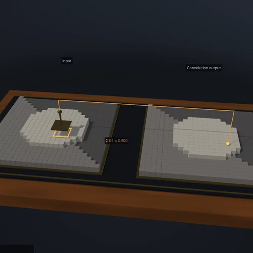
Edit 3×3 image-convolution kernels, inspect individual neighbourhood sums and compare blur, sharpening, edges and embossing.

By Mykhailo Makarov

Actual application image

Try this

Edit all nine kernel coefficients or load a preset. The marked source neighbourhood produces the marked output pixel by true convolution (the kernel is reversed in both axes). Values remain unclipped in readouts; display uses grayscale or a signed colour scale.

Equations used in the module

Equations
(K*I)(x,y) = ΣuΣv K(u,v) I(x−u,y−v)
Mean and Gaussian blur have ΣK=1; Laplacian edge kernel has ΣK=0
Zero, clamped and periodic boundaries give different edge behaviour
The output is not clipped before measurement

Related experiments

Back to catalogue

Math

Least squares and overfitting

Fit noisy data with polynomials, move an outlier, compare training and reference errors and control overfitting with ridge regularization.

Math

k-means clustering

Step through k-means assignments and centroid updates, move centres manually and compare cluster counts on an elbow curve.

Math

Gaussian elimination: planes meeting at a point

Step through Gaussian elimination and its changing equation planes, edit a 3×3 system and examine pivoting and rank.