Engineering
Autonomous shuttle
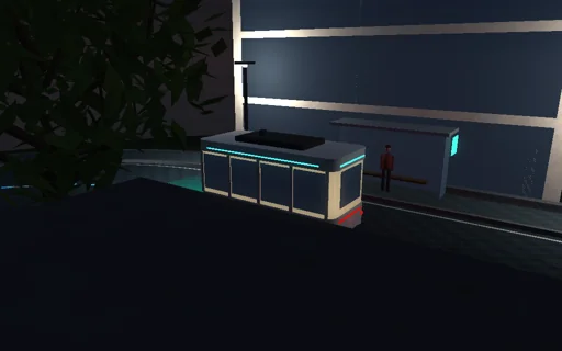
Ride a driverless electric shuttle round a university campus at night after rain. It steers by pure pursuit - aiming at a point ahead on the path with the curvature 2 sin(alpha)/L_d, exactly 1/R on a circle - slows to sqrt(a_lat/kappa) for every curve, stops on the mark at two stations within the comfort limits of deceleration and jerk, and watches the road with a fan of lidar rays. A pedestrian waits at the zebra: the shuttle sees her and yields. Switch the yield rule off and she steps out 14 m ahead - the emergency stop takes the closed-form distance v tau + v^2/2a + v a/2j; give the perception 1.2 s of latency and it reaches her; park a van before the zebra and she stays hidden until she is in the lane. Try dry asphalt and wet leaves, and follow every joule from the battery into motors, air, tyres and brakes and back through regeneration.
What happens
A 3000 kg shuttle (2400 kg and 8 passengers) drives a 116.8 m campus loop, 76 + 13π m, with corners of 5 and 8 m. Kinematic bicycle about the rear axle, wheelbase 3 m: θ’ = v·tan δ/L. Pure pursuit aims at the path point L_d = 2 m + 0.6 s·v ahead and commands κ = 2 sin α/l_d, exactly 1/R on a circle; the steering servo turns at most 0.7 rad/s up to 35°. The planner holds the cruise speed, the curve limit √(a_lat/κ) with a_lat = 1.2 m/s² (never above μg/2) from where the lookahead point enters a curve, and 2 m/s at the zebra while someone waits beside it; for the curves, the next station and an obstacle it brakes once a comfortable slowdown - jerk 1.5 m/s³ down to 0.96 m/s², then constant - needs all the distance left, and then follows v²/2d onto the limit, within 1.2 m/s² and the jerk limit. A 2D lidar on the bumper casts 121 rays over 120° at 10 Hz, range 30 m, noise 2 cm from a fixed seed, against walls, posts, trees, the van and the pedestrian; hits within 1.5 m of the path ahead are obstacles. The planner sees each scan after the latency (0.3 s); if the time to collision is shorter than a comfortable stop needs, it brakes open-loop with jerk 20 m/s³ to min(6, 0.9μg) m/s² and stops in v·τ + v²/2a + v·a/2j − a³/24j² from the scan (μ = 0.85, 0.55, 0.3). Motion is exact piece by piece: constant jerk over at most 10 ms with the steering held is a circular arc of the travelled length; the stop, the end of the brake ramp and the latency instants are found inside the step. Wheel work by four-point Gauss: battery = traction/0.9 + 2 kW auxiliaries − 0.7 × regenerated braking (at most 40 kW), the rest of the braking heats the friction brakes; the ledger closes to round-off.
Try this
Watch a lap: the curve speeds, the station stops on the mark and the shuttle yielding at the zebra; switch the yield rule off and compare the stop with the closed-form distance; raise the latency until the shuttle reaches the pedestrian; choose the van; try wet leaves; shorten the lookahead time and watch the steering.
The model and its limits
A kinematic bicycle: no tyre slip or lateral dynamics, the friction only caps the emergency braking and the curve limit; a teaching planner, not a certified autopilot or a neural network. The lidar scans one plane against circles and segments, without rain clutter, clustering or tracking; the pedestrian follows a script and is never predicted beyond the zebra rule; a contact is flagged, not simulated. The motor or regenerative branch is chosen per 10 ms piece on the net wheel work; the battery is an energy store at constant efficiencies. One campus loop at full scale, no other traffic.
Equations used in the module
Equations
θ’ = v·tan δ/L,  κ_cmd = 2·sin α/l_d,  L_d = L0 + k·v,  on a circle α = L_d/2R, so κ = 1/R
v_curve = √(a_lat/κ),  brake when d ≤ D(v, a, v_c);  then a = −(v² − v_c²)/2d,  |a| ≤ a_c,  |da/dt| ≤ j
TTC = d/v;  emergency if d − 1 m < D_comfort;  s_stop = v·τ + v²/2a_e + v·a_e/2j_e − a_e³/24j_e²,  a_e = min(6, 0.9·μ·g)
E_batt = W_trac/η_m + E_aux − η_r·W_regen,  W_trac − W_brake = ΔE_k + F_r·s + ∫c·v³ dt