Physics
Cart and pole: swing-up and balance
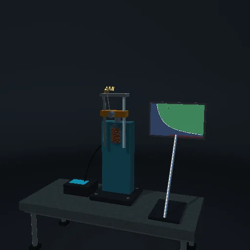
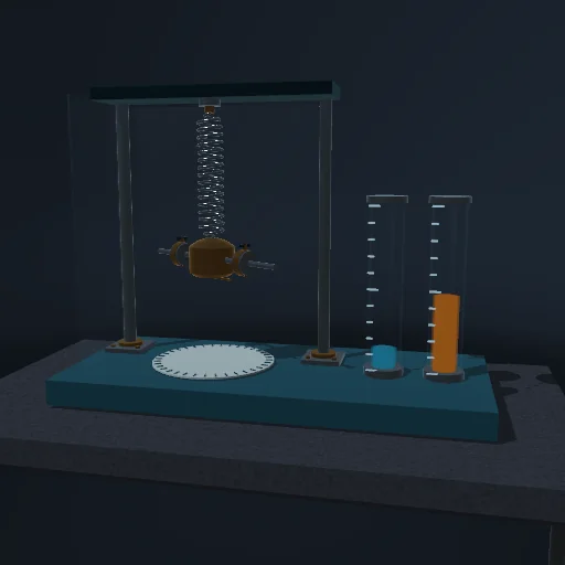
An inverted pendulum on a cart: energy pumping swings it up, a linear-quadratic regulator holds it upright, and a kick shows how the controller recovers. A double pendulum is the hard mode.
What happens
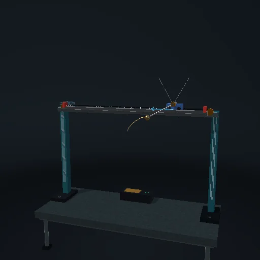
A pole on a cart that can only push the cart left and right - and yet the pole ends up standing on its end. Two laws do it, and the switch between them is the whole story. While the pole hangs, the controller pumps energy: it measures how far the pole's energy is below the upright level and accelerates the cart in the direction that feeds it, the way you time a push on a swing. It aims half an m g l above the top on purpose: aimed exactly at the top, the pole would arrive with nothing to spare and the bearing's friction would keep it a few degrees short forever. Near the ends of the rail the pump fades out and a centring term takes over, so the cart does not reach the end stops. When the pole enters the chalked cone with little enough energy, the law switches: the second law is a linear-quadratic regulator, a fixed gain on the four numbers x, θ, x', θ'. Its gains are not tuned by hand - they come from the Riccati equation of the pole's own equations linearised at the top, solved every time you move a slider. Kick the pole and watch the force under the cart: the regulator recovers from a small kick, and after a large one the pole falls, the first law takes over, and the cycle repeats. Switch the controller off and the pole simply falls. The double pendulum opens standing and is held by the same regulator with six gains; swinging a double pendulum up is trajectory optimisation, and the model does not pretend to it.
Equations used in the module
Equations
(M + m) x'' + m l cos θ · θ'' − m l sin θ · θ'² = F − b x'
m l cos θ · x'' + m l² θ'' − m g l sin θ = −c θ'   (θ from the upright)
E = m l² θ'²/2 + m g l (cos θ − 1),   dE/dt = −m l a θ' cos θ
swing-up:  a = k (E − E_ref) θ' cos θ,  E_ref = 0.5 m g l,  F = (M + m) a,  |F| ≤ 18 N
catch:  |θ| < 30° and E < 0.8 m g l  →  u = −K s,  s = (x, θ, x', θ')
LQR:  AᵀP + PA − P B R^-1 Bᵀ P + Q = 0,  K = R^-1 Bᵀ P,  Q = diag(1, 10, 1, 1),  R = 0.1
linear at the top:  ∂θ''/∂θ = g (M + m) / (M l),  ∂x''/∂θ = −m g / M,  ∂θ''/∂F = −1 / (M l)