Math

Why the bell appears

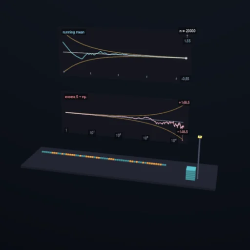
Add up draws from any shape - a die, a loaded coin, two humps, the long tail of a waiting time - and the standardised sum turns into the same bell. One sample is collected before your eyes and becomes one point of the series beside it; the sum, the mean and the standardised sum are three names of that point. Cumulants of a sum add, so the skewness falls as 1/√n and the excess kurtosis as 1/n, and the sheet measures both. And one source breaks it: a Cauchy has no variance, and no bell ever appears.

By Mykhailo Makarov

Actual application image

What happens

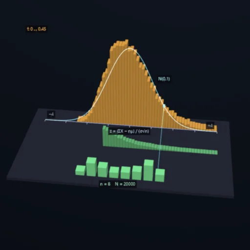
Add up many small independent pieces and the sum falls on the same bell curve whatever the pieces were - that is the central limit theorem, and this module shows it happening and measures how fast. Skewness of the sum dies as 1/√n, excess kurtosis as 1/n: a coin's sum is bell-shaped by a dozen throws, an exponential's lopsided tail needs many more. The exact distribution of the sum is built by convolution and compared with a sampled one and with the normal. Pick a source, raise n, and watch the histogram straighten while the Kolmogorov distance falls.

Equations used in the module

Equations
Z = (X₁ + … + X_n − nμ) / (σ√n)
κ_k(Z) = κ_k(X) / (σ^k n^{k/2−1}):  skewness ∝ 1/√n, excess kurtosis ∝ 1/n
uniform: γ₂ = −6/5;  exponential: γ₁ = 2, γ₂ = 6
Kolmogorov distance to the normal, exact pmf by convolution

Related experiments

Back to catalogue

Math

The average settles, the count does not

A chain you can read - outcome, sum, mean - and two charts on one log-n axis with one cursor: the mean's deviation walks into a funnel of ±2σ/√n, while the excess count S_n − nμ grows like √n and never settles. Predict first whether the excess goes to zero too, then let the run climb; six other runs under the same conditions stand beside it. A forced streak is forgotten by the mean and kept by the count; for the coin the numbers are exact from the binomial; and a Cauchy source, which has no mean, never settles at all.

Math

Ninety-five times out of a hundred

Inspect the observations behind a confidence interval. Repeat the experiment and compare coverage and width of methods on the same samples.

Math

The p-value, and how to fool yourself with it

Two thousand experiments ask whether a mean is zero; the share that rejects at α = 0.05 is counted. With no effect it is 5 % - the type I rate - and the p-values are uniform. With an effect it is the power, which rises with the effect and with n: half a σ is found 32 % of the time with ten observations and 82 % with thirty-four. Look at the data every five observations and stop when p dips below 0.05, and the false positive rate is a quarter. Everything is counted; Student's curve comes from the code.