Math
Linear transformations
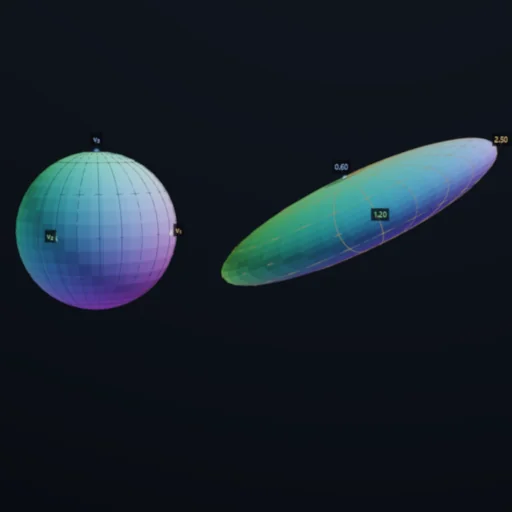
The whole space deformed by a matrix: the unit cube carries the determinant and turns inside out through zero volume, the unit ball becomes the ellipsoid of the singular values, and the eigenvectors are the rods that do not turn.
What happens
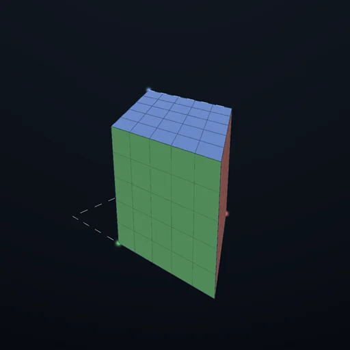
A lattice of lines fills the space; the unit cube stands at the origin with its three faces coloured after the axes; the unit ball sits inside it as a wire sphere; three bright arrows are the images of the axes - the columns of the matrix. The morph g_t = (1 − t)·I + t·A carries all of it from the untouched space to A and back. The lattice shears, the cube becomes the parallelepiped whose signed volume IS the determinant, the ball becomes the ellipsoid whose semi-axes are the singular values. When the determinant is negative the cube has turned inside out and its faces go cold - and it cannot do that without passing through zero volume on the way, which happens at t* = 1/(1 − λ) for each negative eigenvalue λ; the chart shows det g_t along the morph with the zero marked. Glowing rods through the origin are the eigenvectors, the lines A maps onto themselves - warm for a positive eigenvalue, cold for a negative one; a rotation keeps only its axis, because its other two eigenvalues are complex. Every number on the panel is read off the picture - the cube's volume as a triple product, the ball's longest and shortest radius by sampling, the collapse by scanning the morph - and printed beside the closed form. An extra turn about z, applied after the preset, changes neither the determinant nor the singular values, and the panel shows that too.
Equations used in the module
Equations
A is 3 × 3;  det A = a₁ · (a₂ × a₃) - the signed volume of the image of the unit cube (columns a₁, a₂, a₃);  det = 0 ↔ a dimension is lost;  det < 0 ↔ orientation reversed
morph:  g_t = (1 − t)·I + t·A;   det g_t = t³ · det(A + ((1 − t)/t)·I) - zero exactly at t* = 1/(1 − λ) for each real eigenvalue λ < 0
eigen:  A·v = λ·v;   λ³ − (tr A)·λ² + (sum of principal 2 × 2 minors)·λ − det A = 0;   a real 3 × 3 has one or three real eigenvalues;   a rotation keeps only its axis
singular values:  σ² = eigenvalues of A^T·A;   the unit sphere → an ellipsoid with semi-axes σ₁ ≥ σ₂ ≥ σ₃;   max |A·v| = σ₁,  min |A·v| = σ₃ on |v| = 1;   σ₁σ₂σ₃ = |det A|
rank = number of σ > 0;   a rotation R leaves det and σ unchanged:  det(R·A) = det A,  σ(R·A) = σ(A)
presets:  stretch diag(2, ½, 1);  rotation R_z(60°);  shear (x += y);  reflection diag(1, 1, −1);  projection diag(1, 1, 0);  rank one u·v^T;  symmetric [[2,1,0],[1,2,0],[0,0,1]] (λ = 3, 1, 1);  twist·stretch R_z(50°)·diag(1.6, 0.7, 1.2);  negative stretch diag(−2, 1, ½)