Engineering
Wind tunnel balance
Sweep the wing through the stall and read its lift, drag and moment off the strain-gauge balance under the floor, then compare the measured polar with the true one. Calibrate the balance with one weight per channel or with fifteen combined loads, lean its lift links, add noise and shorten the averaging, and see what the cross-talk, the noise and the warming zeros do to the drag.
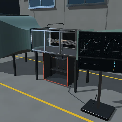
What happens
An open-return wind tunnel draws air through a bellmouth, a honeycomb and screens into a 0.8 × 0.6 m test section and blows it out through a diffuser and an 8 kW fan; its top speed is 35 m/s. With the air's momentum and the losses (K = 0.45) it reaches 99.5 % of 25 m/s in 11.2 s, and the drive then takes 2.90 kW. A rectangular wing of 0.5 m span and 0.1 m chord (aspect ratio 5, a Joukowski section with zero lift at −2.10°) pivots at its quarter chord on a strut that stands on a three-component strain-gauge balance under the floor: the metric frame hangs on two lift links 0.2 m apart and a drag link, each a flexure whose bridge reads its tension. The wing's characteristic has the finite-wing slope 2π·AR/(AR + 2) and Kirchhoff's trailing-edge separation: C_L peaks at 0.942 at 11.2° and falls to 0.595 at 17.6°; L/D peaks at 14.0 at 4.3°. As built, the lift links lean by 1°, the drag link is pitched by 0.3° and the gains differ by up to 3 %, so every bridge reads a mixture of lift, drag and moment.
A run takes the wind-off zero, spins the fan up and sweeps the wing from −4° to 20°. Through the drawing's nominal sensitivities the drag at 4° reads 27 % low, C_D 0.0250 for 0.0341: the lean hands the drag link sin 1° of the lift, 0.157 N of the 0.171 N error, and that error, carried 0.55 m up from the balance centre, turns C_m −0.050 into +0.008. One weight per channel corrects the gains but not the cross-talk: the drag still reads 24 % low. Fifteen combined loads fitted by least squares read the whole sweep true without noise. With 20 µV/V of amplifier noise the drag scatters by 31.6 mN over 10 samples and by half of it over 40. The bridges' self-heating, 3.1 K in two minutes, moves the drag zero by 0.092 N.
Model: quasi-steady aerodynamics from the given characteristic, without wall corrections, Reynolds-number effects or dynamic stall; the balance is one rigid metric body on three pin-ended links in the plane of the flow, with dampers beside them, ringing at 29, 62 and 71 Hz; the weights act as steady forces; the air's density is fixed. RK4 steps end on the amplifier's 1 kHz sample clock, so the readings do not depend on the frame step; the noise is seeded. The tunnel's journal closes (drive = the air's kinetic energy + losses), and so does the balance's (work of the loads = its energy + dampers). The smoke is illustrative: potential flow with the wing's own circulation, lifted over the dead air.
Try this
Watch the sweep draw the polar on the cart: the measured drag falls short of the true curve by the lift the leaning links feed it. Then choose the least-squares calibration, lean the links, add noise or shorten the averaging, and sweep again.
Equations used in the module
Equations
C_L = a·(α − α₀)·((1 + √f)/2)²,  a = 2π·AR/(AR + 2)
C_D = C_D0 + C_L²/(π·e·AR) + (1 − f)·C_D90·sin²(α − α₀)
M·q″ + C·q′ + (K − K_g)·q = Q(L, D, M),  r = s·T_link + r₀ + r_drift + r_noise
F = K_cal·(r − r₀),  K_cal = argmin Σ|F_w − K·(r − r₀)|²