Earth
Continental drift
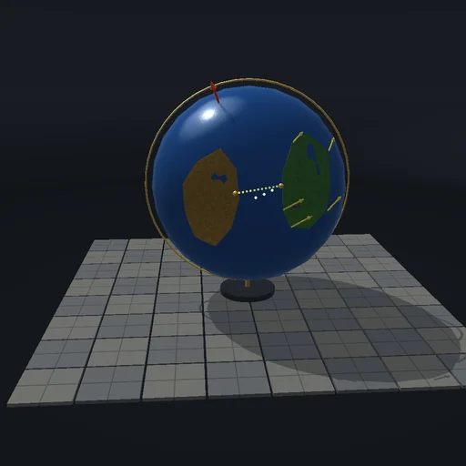
Turn a continent about its Euler pole and watch the ocean open: points near the pole hardly move while those far from it run at full speed, the plate keeps its shape and its area exactly, and the same rotation backwards closes the ocean again. Move the pole, change the rate, give the other plate its own motion and read the opening rate between the coasts.
What happens
Two teaching continents on a globe are rigid plates, each turning about its own Euler pole at its own rate. A contour is placed at time t by Rodrigues’ rotation of its starting vertices, so distances within a plate and the spherical area of its outline (the excess of a fan of spherical triangles) are preserved exactly, and the rotation reversed returns it. A point’s speed is ω·R·sin Δ with Δ its angular distance from the pole; the ocean between two tracked coastal points is measured along the great circle, and its opening rate is the analytic derivative of that distance. Plate boundaries are not computed - this is kinematics on a sphere, not mantle dynamics.
Try this
Run the drift and watch the coast nearest the pole creep while the far end races; read the opening rate, then reverse the rotation and close the ocean. Move plate B’s pole onto the continent to see it spin in place.
The model and its limits
Rigid plates without deformation, Euler poles fixed in the mantle frame, no plate boundaries or spreading ridges; the two continents and their motions are a teaching configuration, not a reconstruction.
Equations used in the module
Equations
r′ = r·cos θ + (k × r)·sin θ + k·(k·r)·(1 − cos θ)
v = ω × r,  |v| = ω·R·sin Δ
tan(E/2) = a·(b × c)/(1 + a·b + b·c + c·a)
d = R·arccos(a·b)