MakarovSuites
English
EnglishDeutschРусскийУкраїнськаFrançaisEspañolItalianoPolski
Contact & licences

Earth

Geothermal gradient

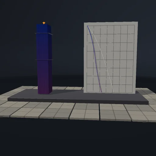
Heat a 40 km column of crust from below at 30 mW/m² while its own radioactivity adds 45 more: the profile curves, steep in the sediments and flatter in the conductive lower crust, and after a few slab time constants of 23 Myr it lands on the closed-form steady state to a hundredth of a degree while the surface heat flow reaches 75 mW/m². Halve the sediments’ conductivity and the whole crust below runs 180 K hotter; double the basal flow and the Moho climbs past 1300 degrees. A uniform half-space after a surface step follows the erf solution. Heat in, made and out balance the stored heat to rounding.
Geothermal gradient — Actual application image
Actual application image

What happens

One-dimensional conduction through a layered crust: eighty finite volumes of half a kilometre with the conductivity and heat production of sediments (2 W/m/K, 1 µW/m³), upper crust (2.5, 2) and lower crust (2.2, 0.5), harmonic face conductivities, the surface held at 10 °C and the base fed 30 mW/m². Explicit stepping at 2 kyr books every face flux and the production, so the stored heat meets what came in, was made and left to rounding; the steady profile is the piecewise-quadratic closed form, and a uniform half-space after a surface step is the erf solution. One second of the experiment is one Myr.

Try this

Watch the profile bend into its steady shape and read the Moho temperature against the closed form; halve the cover’s conductivity, double the basal flow, or start the whole column hot and follow erf.

The model and its limits

Pure conduction with constant properties per layer, no erosion, advection or time-dependent heat production, a fixed basal heat flow. Temperatures are those of this column.

Equations used in the module
Equations
ρc·∂T/∂t = ∂/∂z(k·∂T/∂z) + A,  q = −k·∂T/∂z
k_face = 2k_a·k_b/(k_a + k_b),  q(z) = q_b + ∫_z^L A·dz′
T(z) = T_s + ∫_0^z q/k·dz′,  q_surface = q_b + Σ A·Δz
T(z, t) = T_s + (T_0 − T_s)·erf(z/2√(κt)),  τ = 4L²/π²κ
Related experiments

Back to catalogue
Magnetic reversals — Actual application image

Earth

Magnetic reversals

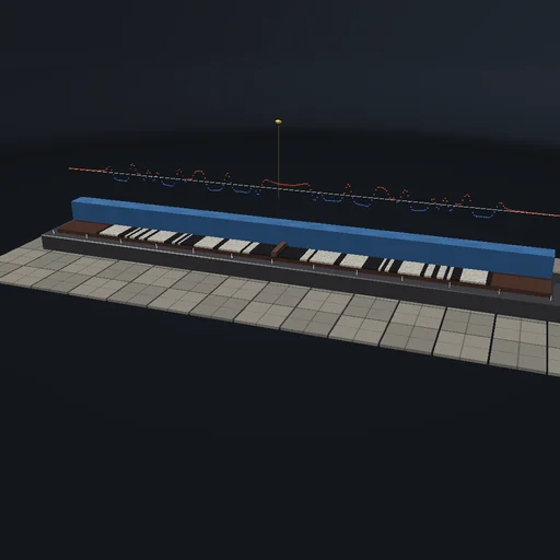
Run a ridge from six million years ago to today at 20 mm/yr and watch the crust leave it in stripes, normal and reversed, each as wide as the spreading rate times the chron it formed in, so the Brunhes stripe spans 15.6 km on each flank and the whole pattern mirrors about the axis. Read the magnetometer’s profile, the thin-sheet anomaly of every stripe summed, symmetric about the ridge; double the rate and the stripes and the profile stretch to match; tow the sensor twice as high and the anomalies blur into one another. The chron table and the block widths are the closed forms.

Glacial rebound — Actual application image

Earth

Glacial rebound

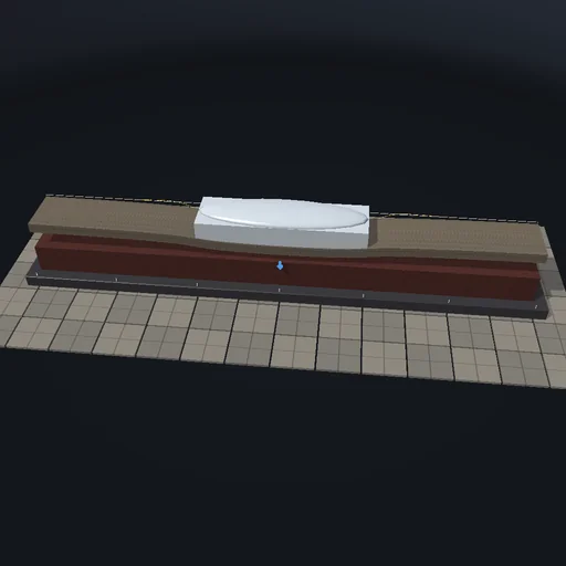
Grow a 1000 km wide, 2 km thick ice sheet over ten thousand years, hold it, melt it in five and watch the land answer: the lithosphere bends as a 50 km elastic plate towards Hetenyi’s bowl, 556 m deep at the centre with a 19 m forebulge 250 km beyond the ice edge, each wavelength of the depression relaxing through the mantle at its own time, three thousand years for the longest. After the melt the centre is still 240 m down and rising at 60 m per thousand years. Thicken the plate and the bowl widens and shallows; double the viscosity and everything takes twice as long; melt gradually and the land never gets far behind the ice.

Water cycle — Actual application image

Earth

Water cycle

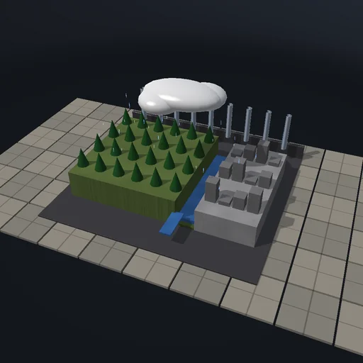
Run a year of weather over a catchment of forest, town and lake: moisture blows in, rains out in proportion to each land’s share, the canopy catches a quarter and breathes it back, forest soil drinks fifty millimetres a day while pavement takes five, soils evaporate and percolate, the groundwater seeps to the river over three hundred days and the river drains to the sea in two. Drop a 50 mm storm on day 100 and compare the flood peak of the forested catchment with the paved one; pump the aquifer hard and watch the baseflow die; cut off the advected moisture and the stores run down together. Nine stores plus exports minus imports keep the initial total to rounding, and the groundwater recession is the closed-form exponential.