Earth
Mountain waves
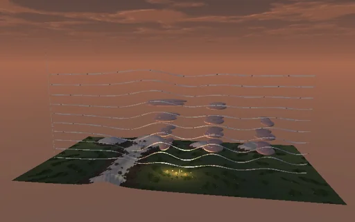
Watch the evening wind cross a snowy ridge: stable air pushed up the windward flank springs back and oscillates downwind, and the steady linear wave field - the Scorer equation solved mode by mode - is drawn as smoke ribbons rising and falling over and behind the ridge. Over a broad ridge in uniform air the waves climb straight up as Queney’s solution, with a vertical wavelength 2πU/N and a drag of (π/4)ρNUh0²; under a less stable layer aloft a train of lee waves is trapped downwind, its crest spacing the closed-form trapped mode, longer as the wind grows, until above a critical speed nothing is trapped. Lenticular clouds stack where moist layers are lifted past their condensation level, a glider climbs in the lift until it equals its sink, and a ridge too high for the wind is flagged where the streamlines would overturn.
What happens
Linear steady two-dimensional Boussinesq flow over a long ridge h(x) = h0·a²/(x² + a²), 600 m high and 2.5 km wide. Each Fourier mode of the streamline displacement η solves the Scorer equation η_zz + (l² − k²)·η = 0 with l = N/U, η = h at the ground and radiation or decay aloft, on a periodic domain of 2048 columns of 400 m (819 km) with the ridge’s exact spectrum π·h0·a·e^(−ka); the mean mode is left out. One layer (uniform N and U) or two: N = 0.015 1/s below 2.5 km and 0.007 above at U = 15 m/s trap one lee-wave mode; there a weak dissipation l²(1 + 0.03i) lets the train decay downstream (e-folding about 60 km) instead of wrapping round. Every 250 m level is an inverse FFT; the drag is ρ·U²·∫η_x·η_z dx at the ground, the momentum flux the same integral aloft, the energy flux U times the drag. Upstream the temperature falls at g/c_p − N²T/g; moist layers 500 m thick every 1.5 km up to 6 km carry the set humidity, the air between 0.55 of it; a parcel lifted past 125 m per kelvin of dewpoint depression condenses. Tracers drift at U(1 − η_z) in 5 s steps; the glider holds its ground position in the strongest lift at its height and climbs at w − 0.9 m/s.
Try this
Raise the wind and read the lee-wave crest spacing against the closed form; push it past the critical speed; make the air uniform and the ridge broad for Queney’s waves; raise the ridge until the streamlines overturn; moisten the air for lenticular clouds; release the glider.
The model and its limits
Linear, steady, two-dimensional and Boussinesq: no rotors, wave breaking, blocking or hydraulic jumps - past N h0/U ≈ 1 the model only flags the overturning; a uniform wind; a weak artificial dissipation in the two-layer case; clouds are a saturation test of lifted parcels, with no latent heat or precipitation. The glider and the village are drawn twenty times larger.
Equations used in the module
Equations
η_zz + (l² − k²)·η = 0,  l = N/U,  η(x, 0) = h0·a²/(x² + a²)
η = h0·a·(a·cos lz − x·sin lz)/(x² + a²),  λz = 2πU/N,  D = (π/4)·ρ·N·U·h0²
m1·cos(m1·H) + μ·sin(m1·H) = 0,  m1² = l1² − k²,  μ² = k² − l2²,  λ = 2π/k
D = ρ·U²·∫η_x·η_z dx,  w = U·η_x,  cloud where η ≥ 125 m/K·(T − T_d)