Earth
Air pollution dispersion
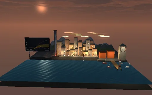
Watch the smoke of a brick factory chimney drift over a terraced town at dawn. The hot exhaust rises by Briggs’s plume rise, then the wind carries it downwind while the turbulence of the chosen Pasquill class mixes it towards the ground: in a sunny unstable morning it loops down within a few hundred metres, in a neutral one it touches the town a couple of kilometres away, in a calm stable night it fans out aloft and barely reaches the roofs. Let an inversion lid trap it over the houses, or set the lid below the plume and the town stays clean. A ribbon over the roofs draws the ground-level concentration beside the Gaussian plume, a station reads it; with a uniform wind and a constant K the slab settles onto the exact steady plume, its ground maximum 2Q/(eπuH²). Stop the source and watch what is left blow out of the valley; the emitted mass always equals what is in the air, deposited and gone.

What happens
An 80 m chimney 3 m across releases 100 g/s at 12 m/s and 150 °C into 5 °C air: buoyancy flux F = g·w·d²·ΔT/(4·T_s) = 90.8 m^4/s^3, Briggs’s final rise 38.71·F^0.6/u = 69 m in class D (2.6·(F/(u·s))^(1/3) = 52 m in class F), reached by the 2/3 law 1.6·F^(1/3)·x^(2/3)/u at 119·F^0.4 = 722 m. From the effective height H the crosswind-integrated concentration is carried by the urban power-law wind u10·(z/10)^p and mixed by K(z) = κ·u*·z·(1 − z/h)²/φ_h(z/L) (z0 = 1 m, mixing heights 1600 m for A down to 220 m for F) in a slab 3 km long and 1 km high, 120 × 100 cells of 25 × 10 m: upwind advection at CFL ≤ 1, the release split between two cells so its centroid is exactly H, then four backward-Euler mixing sub-steps per column with dry deposition 0.5 cm/s at the ground, an optional inversion lid with K = 0 and an open top. The axis concentration is C_y/(√(2π)·σ_y) with the Briggs urban σ_y. The Gaussian reference uses the Briggs urban σ_y and σ_z with the ground’s and lid’s images; its maximum is found by a log scan and golden section. With a uniform 5 m/s wind and K = 25 m²/s the slab reproduces the steady image solution to 0.5 % and the ground maximum 2Q/(eπuH²) at uH²/4K; each column’s variance grows by exactly 2K·t. Emitted = in the air + deposited + left through the downwind face and the top, to rounding.
Try this
Step through the classes from A to F and watch the plume loop, cone and fan; drop an inversion lid onto it, then below it; change the wind while it runs; stop the source and let the cloud leave; switch to uniform K and compare the ribbon with the Gaussian line.
The model and its limits
A passive gas in a two-dimensional slab along the wind with a Gaussian crosswind spread, flat ground, steady profiles for each class, final rise released at the stack, no chemistry or wet removal. The Gaussian reference carries the Briggs urban spreads, which mix faster near the stack than surface-layer K-theory, so the two differ - by about two at class D and far more on a stable night. Smoke seen is not a toxicity scale.
Equations used in the module
Equations
F = g·w·d²·(T_s − T_a)/(4·T_s),  Δh = 38.71·F^0.6/u (neutral),  Δh = 2.6·(F/(u·s))^(1/3) (stable)
∂C/∂t + u(z)·∂C/∂x = ∂/∂z(K(z)·∂C/∂z),  K·∂C/∂z = v_d·C at the ground,  K = 0 at the lid
K(z) = κ·u*·z·(1 − z/h)²/φ_h(z/L),  u(z) = u10·(z/10)^p,  c = C_y/(√(2π)·σ_y)
c(x,0,0) = Q/(π·u·σ_y·σ_z)·e^(−H²/2σ_z²);  constant K: c_max = 2Q/(e·π·u·H²) at x = u·H²/(4K)