Earth
Vegetation, water and climate
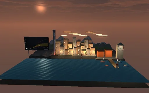
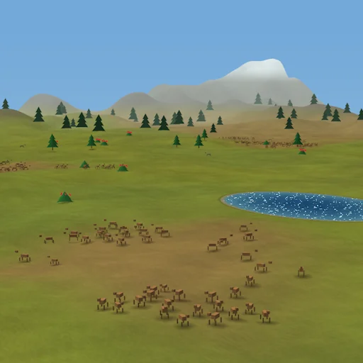
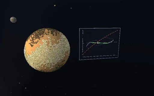
Walk around a little planet covered with daisies as its sun grows brighter. Black daisies absorb sunlight and warm themselves and the planet, white ones reflect it and keep cool; both grow best at 22.5 °C. So the faint young sun is met by black daisies, the bright old one by white ones, and in between both together hold the planet within a few degrees of the optimum while the bare planet would warm by forty - the closed-form coexistence branch on the board, its local temperatures exactly 5 K either side of the optimum. Push the sun past 1.54 and the whites collapse in one jump; dim it again and they return only at 1.22 - sweep and watch the hysteresis drawn. Switch to the desert: plants bring their own rain, and at the same rainfall a green savanna and a bare desert are both stable, until a drought tips the green one over for good. Areas are booked to round-off.
What happens
Daisyworld after Watson and Lovelock: white daisies (albedo 0.75), black daisies (0.25) and bare ground (0.5) share the planet, a_w + a_b + x = 1. The planetary albedo A sets the emission temperature σT_e⁴ = S·L·(1 − A) with S = 917 W/m² and the luminosity L; heat is shared only partly, so each patch sits at T_i = q’(A − α_i) + T_e with q’ = 20 K. Each kind grows on bare ground at x·β(T_i) − γ with β = 1 − 0.003265·(T_i − 22.5 °C)², zero at 5 and 40 °C, and dies at γ = 0.3 per year; the three areas are stepped together by RK4 at 0.1 year, so their sum stays 1 to round-off. A kind that dies back keeps a dormant seed bank of 1 %; the moment it reaches it is found inside the step. Together the two kinds can only stand still where both grow alike: their patches 5 K either side of the optimum, bare ground x* = γ/β = 0.327, and L an explicit function of A - the regulated branch from L = 0.744 to 1.342 on which T_e falls from 25.8 to 19.2 °C while the bare planet would warm from 5.8 to 49.3 °C. Seeds germinate on a bare planet at L = 0.718 (blacks) and only below 1.221 (whites); one kind alone dies at the fold of its explicit branch, 0.629 for blacks, 1.545 for whites - hence the hysteresis. The desert experiment follows Charney and Brovkin: rainfall P = P_d + k·V with k = 350 mm/yr from the plants’ own recycling and darker ground, the cover relaxing over 25 years to the ramp V* = (P − 100)/(400 − 100) clamped to 0…1. With k larger than the ramp’s width both bare sand and full cover are stable for desert rain between 50 and 100 mm/yr, split by an unstable middle; departures from it grow as e^(λt), λ = 1/150 per year, and the kinks of the ramp are located inside the step.
Try this
Watch the daisies bloom from seeds and cool the planet to 21.9 °C while the bare planet would stand at 26.7 °C; move the sun and read the regulated temperature against the closed form; press the sweep and draw the hysteresis loop on the board. Switch to the desert, set the rain without plants to 75 mm/yr and try a green and a bare start; lower the rain below 50 mm/yr, or clear the savanna, and watch it not come back.
The model and its limits
A zero-dimensional Daisyworld with the linear local-temperature law (q’ = 20 K) instead of a full heat transport, no heat capacity, a fixed 1 % seed bank, two kinds of daisy and no evolution; their placement over the globe (whites towards the equator, blacks towards the poles) is presentation, the model’s areas are global. The savanna is one box with a linear rainfall recycling and a piecewise-linear ramp of cover, not the two plots with soil water and surface energy fluxes the design plans for a later stage. Thresholds belong to these teaching models, not to the Earth’s history.
Equations used in the module
Equations
σ·T_e⁴ = S·L·(1 − A),  A = a_w·α_w + a_b·α_b + x·α_g,  a_w + a_b + x = 1
T_i = q’·(A − α_i) + T_e,  β(T) = 1 − k·(T − T_opt)²,  da_i/dt = a_i·(x·β(T_i) − γ)
coexistence: T_b,w = T_opt ± q’·(α_w − α_b)/2,  x* = γ/β,  L = σ·T_e(A)⁴/(S·(1 − A))
P = P_d + k·V,  dV/dt = (V*(P) − V)/τ,  V_m = (P_d − P_s)/(P_f − P_s − k)