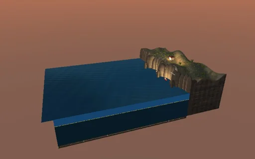
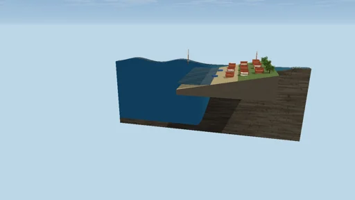
Earth
Density drives the ocean
Watch the Atlantic overturn, cut open from the tropics to the Arctic: warm salty water runs north on top, gives its heat to the polar air, grows dense and sinks in the Nordic Seas, and returns south along the bottom - Stommel’s two boxes joined by the flow q = K(αΔT − βΔS). Cold makes the polar water denser, fresh water makes it lighter: melt the Greenland ice sheet and the overturning weakens along a closed-form equilibrium curve until, past the critical freshwater flux of 0.66 Sv, no thermal state is left and the circulation collapses within centuries, reverses and carries only a fraction of the heat north. Take the meltwater away and it does not come back - it recovers only once the north turns net evaporative. Sweep the flux slowly up and down and trace the hysteresis loop on the board; salt and heat are booked to round-off.
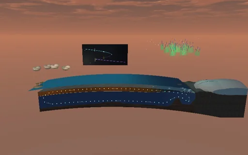
What happens
Two boxes of 10^17 m³ each - the tropical and the polar Atlantic - are joined at the surface and at depth by the flow q = K(αΔT − βΔS) with K = 6500 Sv, α = 1.7·10^-4 per K and β = 7.6·10^-4 per psu; q is positive when the polar water is denser and sinks. Each box’s temperature relaxes over 5 years to its air, 25 °C in the tropics and 5 °C in the north; the freshwater flux F to the north (0.35 Sv plus Greenland meltwater, balanced by evaporation in the tropics) acts as a virtual salt flux F·S0 with S0 = 35 psu, and |q| exchanges heat and salt between the boxes. Salt is conserved exactly, and the heat content changes only by the air-sea flux integrated with the same RK4 weights, so both ledgers close to round-off; the meridional heat transport is ρ·c_p·|q|·ΔT, 1.36 PW today. Every equilibrium lies on the explicit curve F(q) = |q|(αΔT(q) − q/K)/(β·S0) with ΔT = ΔT*/(1 + 2τ|q|/V): the thermal branch folds at q = 10.4 Sv and F_c = 0.66 Sv (Cardano’s root of a cubic; with fixed temperatures K·α²·ΔT*²/(4β·S0) = 0.71 Sv), and the reversed haline branch ends at F = 0, so between the two the ocean remembers its past. Fixed RK4 steps of a quarter year; a change of sign of q inside a step, where |q| has its kink, is located by bisection and integrated exactly to it, and the freshwater sweep turns exactly at its bounds. With fixed temperatures (Stommel’s limit) the salinity contrast obeys a Riccati equation, so the collapse and recovery times are arctan and log closed forms, and a slow sweep collapses past the fold by the Airy delay 2.338·(A²·b)^(-1/3).
Try this
Start from today’s overturning and add Greenland meltwater: 0.2 Sv weakens it, 0.5 Sv takes it past the fold and it collapses after about 570 years. Take the melt away and it stays collapsed; set the freshwater flux below zero to bring it back. Press the sweep and trace the hysteresis loop on the board; switch to fixed temperatures for Stommel’s exact limit.
The model and its limits
Two well-mixed boxes of equal volume, a linear equation of state, temperatures relaxed to fixed air temperatures, freshwater as a virtual salt flux; no wind-driven gyres, no geography, no third (Rooth) box, no sea-ice physics - the ice drawn follows the heat transport. Thresholds and times belong to this teaching model, not to the real Atlantic.
Equations used in the module
Equations
q = K·(α·(T_e − T_p) − β·(S_e − S_p)),  q > 0: sinking in the north
dT_e/dt = (T_e* − T_e)/τ − |q|·ΔT/V,  dT_p/dt = (T_p* − T_p)/τ + |q|·ΔT/V
dS_e/dt = −dS_p/dt = (F·S0 − |q|·ΔS)/V,  H = ρ·c_p·|q|·ΔT
F(q) = |q|·(α·ΔT*/(1 + 2τ|q|/V) − q/K)/(β·S0),  F_c = K·α²·ΔT*²/(4β·S0) at fixed T