Engineering
Flapping-wing flying machine
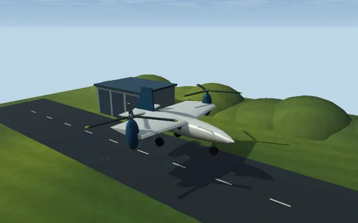
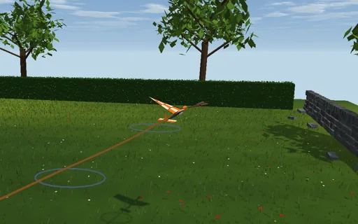
Fly a radio-controlled ornithopter over a summer meadow: a crank flaps two fabric wings of 1.2 m span four times a second and twists them as they beat, and every strip of each wing gets its lift and drag from the air it meets - the forward speed plus its own flapping velocity. Twist the wing nose-down through the downstroke and the lift leans forward into thrust; let the twist lag a quarter of a stroke and the wing only drags; take the twist away and it stalls. On the test stand the balance shows the cycle-averaged thrust, lift and motor power, and the efficiency peaks at a Strouhal number f·A/U near 0.34, inside the band 0.2-0.4 where birds cruise. In free flight the autopilot holds the height with the elevator; add a 50 g payload and the height sags, 100 g brings the machine down on the meadow unless it flaps faster. Every joule of the motor goes into the air, the height and the speed.
What happens
A 0.32 kg ornithopter (pitch inertia 0.006 kg·m²) with two rectangular fabric half-wings, b = 0.6 m by c = 0.25 m, hinged on the body axis 1 cm ahead of the centre of mass. The crank flaps them as φ = φ0·sin S, S’ = 2πf, φ0 = 25°, and twists each strip by (r/b)·Θ·cos(S − ψ), Θ = 40° at the tip, so with ψ = 0 the wing is nose-down through the downstroke. Each of 12 strips per wing meets the air at its own velocity - the body’s, the pitch rate’s and the flapping r·dφ/dt - and its angle of attack α = 4° + twist − atan2(v_n, v_x) gives C_L = σ·4.4·α + (1 − σ)·sin 2α and C_D = 0.03 + 0.083·C_L² + (1 − σ)·2·sin²α, σ = 1/(1 + (α/0.24)^8): attached flow blended into a flat plate past the stall. A 0.05 m² tailplane 0.45 m behind (slope 3.3) carries the elevator; the altitude hold adds 0.02 rad per metre below 6 m and 0.06 rad per m/s of sink, within ±20°; body drag area 0.004 m². Forces are held over sub-steps of at most 1 ms, cut exactly at the end of each stroke and at touchdown, with Euler velocities and trapezoid positions, so the motor’s work −Σ f_n·r·Δφ equals the air’s work plus the kinetic and potential energy (plus the stand’s work T·U·t) to round-off. On the stand the airframe is held in a steady wind and the balance gives the cycle means. Closed forms: St = f·2b·sin φ0/U; the momentum-theory ideal power 2W²/(ρ·U·π·(2b)²); the linear small-amplitude thrust ρ·U·c·a·(b³/6)·φ0·ω·(φ0·ω/U − Θ·cos ψ/b) less the mean drag; the motor-off glide trim from the moment balance.
Try this
On the stand turn the twist lag: the thrust is positive only within about ±45° of nose-down through the downstroke; take the twist away and the wing stalls, give it 60° and it windmills; sweep the frequency and watch the efficiency peak inside the Strouhal band 0.2–0.4. In flight add 50 g and then 100 g of payload and flap faster to carry it; stop the motor to glide.
The model and its limits
Quasi-steady strips with explicit teaching CL and CD curves: no added mass, no wake induction or Wagner lag, no leading-edge vortex, no dynamic stall, no membrane elasticity; the twist is prescribed kinematics, the wings are massless and the air is still. The flight is longitudinal only (distance, height, pitch) and is drawn along a circle round the pilot without modelling the turn. The numbers belong to this idealized machine, not to a real ornithopter.
Equations used in the module
Equations
α = i + (r/b)·Θ·cos(S − ψ) − atan2(v_n, v_x),  v_n = w·cos φ + r·dφ/dt,  φ = φ0·sin S
dF = ½·ρ·|v|²·c·dr·(C_L·e_L − C_D·e_v),  C_L = σ·a·α + (1 − σ)·sin 2α,  σ = 1/(1 + (α/α_s)^8)
St = f·A/U,  A = 2b·sin φ0;   P_ideal = 2W²/(ρ·U·π·(2b)²)
W_motor = −Σ f_n·r·Δφ = W_air + ΔE_k + ΔE_p (+ W_stand)