MakarovSuites
English
EnglishDeutschРусскийУкраїнськаFrançaisEspañolItalianoPolski
Contact & licences

Earth

Folding of strata

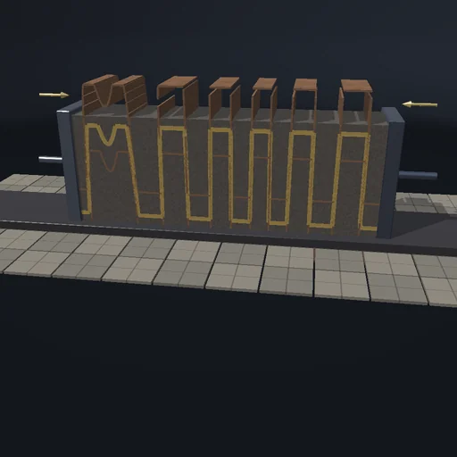
Squeeze a 100 m sandstone bed a hundred times stiffer than its shale along its length: every wavelength seeded in it grows, but the one near Biot’s 2 pi h (eta_l / 6 eta_m)^(1/3) grows fastest and the bed buckles into regular folds, their amplitude the exponential of the growth integrated over the shortening history. Double the thickness and the folds double in wavelength; raise the contrast and they lengthen as the cube root; take the contrast away and the bed only thickens with its matrix. The viscous power of the shortening is read in watts per metre of fold.
Folding of strata — Actual application image
Actual application image

What happens

A stiff layer in a softer matrix under layer-parallel shortening, in Biot’s theory: the layer’s shape is a sum of 96 cosine modes on a 24 km domain seeded with metre-scale incoherent amplitudes; each mode grows at the kinematic rate of plane-strain shortening plus the Biot rate 4(η_l − η_m)·ε·h·k/(η_l·h³·k³/3 + 4η_m), while the domain shortens and the layer thickens as e^(εt) so every wavenumber drifts. The mode that wins sets the measured wavelength, compared with Biot’s dominant wavelength 2π·h·(η_l/6η_m)^(1/3); each mode’s amplification is also the exponential of the quadrature of its rate. One second of the experiment is one Myr; the run stops at 50 percent shortening.

Try this

Watch the noise sort itself into folds of one wavelength and read it against Biot’s; double the thickness, raise or remove the contrast, and compare.

The model and its limits

Linear (small-amplitude) theory carried to visible amplitudes, Newtonian viscosities, a single layer without gravity, detachment or fracture. Wavelengths are those of the linear selection.

Equations used in the module
Equations
dA_k/dt = (ε + q_k)·A_k,  q = 4(η_l − η_m)·ε·h·k/(η_l·h³·k³/3 + 4η_m)
k(t) = k_0·e^(εt),  h(t) = h_0·e^(εt),  L(t) = L_0·e^(−εt)
λ_d = 2π·h·(η_l/6η_m)^(1/3)
A(t) = A_0·exp(∫(ε + q(k(t), h(t)))·dt),  P = 4η_l·ε²·h·L
Related experiments

Back to catalogue
Metamorphism — Actual application image

Earth

Metamorphism

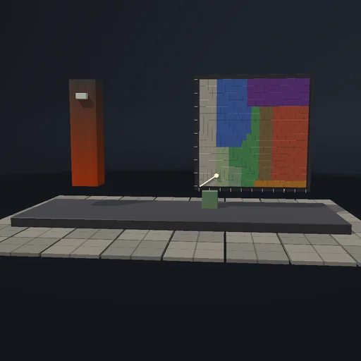
Bury a shale at a kilometre per million years down a 25 K/km geotherm, hold it, and lift it back: its point moves across the pressure-temperature grid of facies, chlorite gives way to biotite, garnet and staurolite as the equilibrium shares shift, and because the reaction rate falls a thousandfold between 600 and 400 degrees the peak assemblage is carried to the surface almost untouched, a little more retrograded when the exhumation is slow. Steepen the burial under a cold gradient and the path runs into blueschist; let a pluton heat a shallow rock and it bakes to hornfels; hold a sample isothermal and its shares relax on the closed-form exponential.

Geothermal gradient — Actual application image

Earth

Geothermal gradient

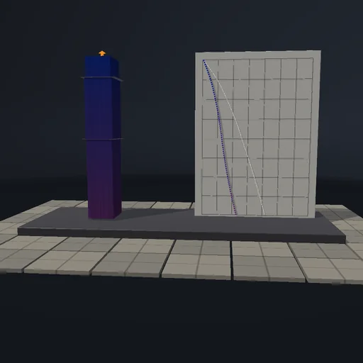
Heat a 40 km column of crust from below at 30 mW/m² while its own radioactivity adds 45 more: the profile curves, steep in the sediments and flatter in the conductive lower crust, and after a few slab time constants of 23 Myr it lands on the closed-form steady state to a hundredth of a degree while the surface heat flow reaches 75 mW/m². Halve the sediments’ conductivity and the whole crust below runs 180 K hotter; double the basal flow and the Moho climbs past 1300 degrees. A uniform half-space after a surface step follows the erf solution. Heat in, made and out balance the stored heat to rounding.

Magnetic reversals — Actual application image

Earth

Magnetic reversals

Run a ridge from six million years ago to today at 20 mm/yr and watch the crust leave it in stripes, normal and reversed, each as wide as the spreading rate times the chron it formed in, so the Brunhes stripe spans 15.6 km on each flank and the whole pattern mirrors about the axis. Read the magnetometer’s profile, the thin-sheet anomaly of every stripe summed, symmetric about the ridge; double the rate and the stripes and the profile stretch to match; tow the sensor twice as high and the anomalies blur into one another. The chron table and the block widths are the closed forms.