Earth
Midlatitude cyclone
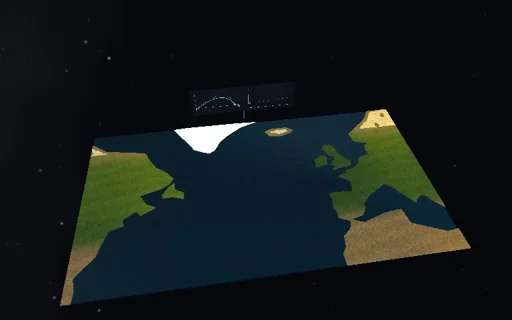
Watch a storm being born over the North Atlantic, seen from orbit. Cold air to the north and warm air to the south mean, by the thermal wind, a westerly wind that strengthens with height - and that sheared flow is unstable. A ripple of half a hectopascal grows exponentially, at exactly the rate the two-layer Phillips model gives in closed form, fastest for waves about 3.5 Rossby radii long, some 4000 km; in a few days lows deepen below 985 hPa, highs build, the comma cloud rises where the warm air climbs ahead of each low and a cold-front band trails behind it. The growth stops when the storms have carried enough heat poleward to slacken the gradient. Flatten the temperature gradient and the wave only decays; compare two wavelengths started alike; the board plots the growth rate against wavenumber and books the eddy energy against its release from the mean available potential energy.
What happens
Two layers of 5 km under a rigid lid at 45° N (f0 = 1.03·10^-4 1/s, N = 0.012 1/s, deformation radius 582 km, Rossby radius of the full depth 1164 km) fill a channel 8000 km long and 4000 km wide, periodic from west to east, with walls in the south and north. A temperature drop of 10 K per 1000 km imposes, by the thermal wind, a shear of 18.3 m/s between the layers over a resting lower layer. The perturbation potential vorticity of each layer, q = ∇²ψ ± F·(ψ2 − ψ1), is carried by the imposed and the eddy winds; the lower layer feels Ekman drag with a 4-day spin-down, the temperature relaxes to the imposed gradient in 20 days, a viscosity of 10^5 m²/s takes the enstrophy at the grid scale. 64 × 32 points of 125 km, Arakawa’s energy-conserving Jacobian, the inversion spectral in x and tridiagonal in y, RK4 at 20 minutes. Every Fourier mode with the wall-to-wall sine is an exact eigenvector of these equations: its growth is the larger root of a 2 × 2 complex eigenproblem - 0.579 per day for the 4000 km wave, 0.406 for 8000 km - and without friction Phillips’ formula σ = k·U·√((2F − K²)/(2F + K²)), largest, (√2 − 1)·U·√(2F) = 0.80 per day, at 3.45 Rossby radii. The eddy energy grows by the release C of mean available potential energy, proportional to the poleward heat flux, and loses to drag, viscosity and relaxation; integrated with the RK4 weights, the ledger keeps only the integrator’s truncation, a few 10^-8 of the energy. Clouds stand where the diagnosed mid-level ascent exceeds 3 mm/s; the isobars are the lower layer’s pressure ρ·f0·ψ2 read as surface pressure.
Try this
Run the 4000 km wave and compare the measured growth on the board with the closed form; let it saturate into 980 hPa lows and watch the heat transport overshoot; start the 8000 km wave alike; set the gradient to zero; start from noise and see the fastest wave take over.
The model and its limits
A quasi-geostrophic two-layer channel on an f-plane: no β effect, no moisture or latent heat, no fronts sharper than the 125 km grid, lows and highs mirror each other; the imposed shear is uniform across the channel and the walls are rigid. Clouds and pressures are diagnostics of this idealized storm, not a forecast.
Equations used in the module
Equations
q1 = ∇²ψ1 + F·(ψ2 − ψ1),  q2 = ∇²ψ2 + F·(ψ1 − ψ2),  F = f0²/(N·H)²
∂q/∂t + J(ψ, q) + U·∂q/∂x ± F·ΔU·∂ψ/∂x = ν·∇²(∇²ψ) − r·∇²ψ2 ± F·(ψ1 − ψ2)/τ_R
ΔU = g·H·(−dT/dy)/(f0·T0),  σ = k·(ΔU/2)·√((2F − K²)/(2F + K²)),  σ_max = (√2 − 1)·(ΔU/2)·√(2F)
dE/dt = C − D,  C = (F·ΔU/2)·mean(ψ1·∂ψ2/∂x) = (F·ΔU/2)·(g·H/(f0·T0))·mean(v·δT)