Math
Vector fields
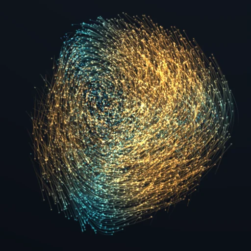
Thousands of tracers reveal a three-dimensional field with luminous fading paths. Orbit the cloud, change its field and emitter, then measure divergence, curl, flux and circulation.
What happens
Thousands of tracers reveal a three-dimensional field with luminous fading paths. Orbit the cloud, change its field and emitter, then measure divergence, curl, flux and circulation.
Passive markers solve dx/dτ = F(x), not acceleration or a charged-particle equation. The six fields are steady: paths follow streamlines. Pace differs by field; rate changes τ, never normalizes the local vector. ABC can contain both tangled and ordered paths. The softened dipole is the existing illustrative field with r² + 0.05, not an exact vacuum magnetic dipole. Markers leaving the displayed domain or their 6–12 s lifetime are released again; old and new paths never join. Emission and brightness are artistic, not fluid density, luminosity or a conserved particle count. Colour uses a bounded speed mapping. Fade and width are display controls. Flux/circulation use the original field, independently of the cloud. The finite grid has quadrature error. The reference box spans ±2; tracers stay in a ball of radius π (dipole 2). Camera drag switches automatic orbit off.
Equations used in the module
Equations
div F = ∂F_x/∂x + ∂F_y/∂y + ∂F_z/∂z;   curl F = (∂F_z/∂y − ∂F_y/∂z, ∂F_x/∂z − ∂F_z/∂x, ∂F_y/∂x − ∂F_x/∂y)
Gauss:  ∫ F·dA over a closed surface = ∫ div F dV over the inside
Stokes:  ∫ F·dl round a loop = ∫ curl F·dA over the disc it bounds
ABC:  F = (A sin z + C cos y, B sin x + A cos z, C sin y + B cos x),  curl F = F,  div F = 0
particles:  dx/dt = F(x), integrated by Runge–Kutta 4