Earth
Carbon through Earth systems
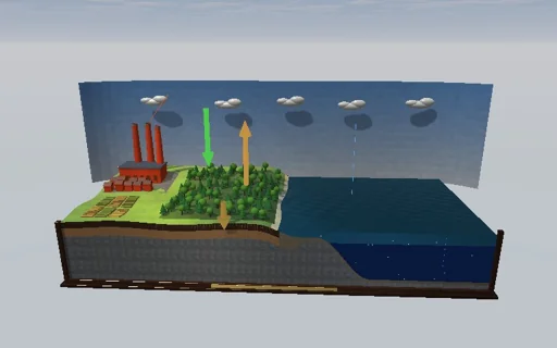
Follow every petagram of carbon through a museum relief of the Earth: chimneys burn fossil carbon into the air, the forest draws it down and drops it into the soil, the soil breathes it back faster as the world warms, and the ocean dissolves it - first the thin surface layer, whose buffer chemistry takes only a tenth of what its size suggests (the Revelle factor), then over centuries the deep ocean. Replay the industrial era: 667 PgC by 2025 bring CO2 to 426 ppm with 47 % still airborne; hold the emissions and CO2 passes 580 ppm by 2100, reach net zero in 2050 and it falls back towards 329 ppm. Release the same carbon at once or over two centuries, clear the forest, and watch the cycle share it out again: the multi-exponential response of the linearised cycle, its equilibrium partition and an exact carbon ledger are shown beside it.
What happens
Five reservoirs in PgC: the atmosphere A (A0 = 595 PgC = 280 ppm at 2.124 PgC per ppm), the surface ocean M (900), the deep ocean D (37 100), the forest B (550) and the soils S (1500). The air and the surface water exchange 60 PgC/yr each way; the net flux F_as = (60/A0)(A − A0·(M/M0)^R) closes once the water’s CO2 pressure matches the air, and with the Revelle factor R = 10 the pressure rises ten times faster than the dissolved carbon. The surface mixes with the deep at F_sd = (M − M0·D/D0)/10 yr. The forest grows NPP = 60·(1 − f)·(1 + β·ln(A/A0)) PgC/yr with β = 0.4, its litter turns over in 9.2 years, the fields on the cleared share f put 60 % of the forest’s production straight into the soil, and the soil respires S/25 yr times Q10^(ΔT/10), Q10 = 2, ΔT = 2 K per doubling of CO2. Emissions: a pulse (instant or spread), or 11 PgC/yr in 2025 reached by an exponential ramp from 1850 (65-year e-folding), then held or cut linearly to net zero; clearing burns the cut vegetation at once. Fixed RK4 steps of 1/32 year hit every kink of the scenario; the rates sum to the emissions, booked with the same weights, so the carbon ledger closes to round-off. Linearised at preindustrial, the cycle is x′ = Jx + E: a pulse decays as Σ r_i·e^(λ_i·t) over the eigenvalues of J - zero (12.1 % stays airborne for good), the deep ocean’s 125 years, the land loop’s damped 11.5 years and the air-sea 1.2 years - with residues from the adjugate, and every scenario is convolved with it in closed form.
Try this
Start with the history and net zero by 2050: CO2 peaks at 442 ppm in 2038 and falls to 386 ppm by 2100; once emissions end, the level it would settle at stays 329 ppm. Choose the pulse: 1000 PgC at once jumps to 751 ppm, the same over 200 years peaks at 446 ppm - and both end at 342 ppm. Drag the cleared share up during a run to burn part of the forest; switch to the linearised cycle to see the closed form match the model exactly.
The model and its limits
A five-box teaching model of the global cycle: one well-mixed surface ocean with a constant Revelle factor (no carbonate chemistry, alkalinity or pH, no dissolution of sea-floor carbonate, so 12 % of a pulse stays airborne for good), one deep ocean, one forest and one soil box; warming follows CO2 at once through a fixed sensitivity, with no ocean heat lag and no other climate response; no permafrost, fire regimes, nitrogen limits or volcanic and weathering fluxes over millennia. Fields hold no vegetation of their own. Numbers belong to this model, not to a carbon budget.
Equations used in the module
Equations
dA/dt = E − F_as − NPP − C + R_h,  dM/dt = F_as − F_sd,  dD/dt = F_sd,  dB/dt = NPP − B/τ_B,  dS/dt = B/τ_B + C − R_h
F_as = (F0/A0)·(A − A0·(M/M0)^R),  F_sd = (M − M0·D/D0)/τ_mix
NPP = NPP0·(1 − f)·(1 + β·ln(A/A0)),  R_h = (S/τ_S)·Q10^(ΔT/10),  ΔT = W·log2(A/A0)
A − A0 = P·Σ r_i·e^(λ_i·t),  r_0 = 1/(1 + (M0 + D0)/(R·A0) + (β·B0 + (β − κ)·S0)/A0)