MakarovSuites
English
EnglishDeutschРусскийУкраїнськаFrançaisEspañolItalianoPolski
Contact & licences

Earth

Ice and albedo feedback

Watch a planet’s ice caps in the light of its sun: each latitude band absorbs sunlight according to its albedo, radiates to space and shares heat with its neighbours. Today’s sun puts the ice edge near 66 degrees; dim it slowly and the edge creeps towards the equator until, at nine tenths of today’s sunshine, the bright ice reflects so much that the whole planet freezes over in one jump. Brighten the sun again and the snowball stays frozen far past where it froze - it thaws only at more than six fifths. Make ice and water equally dark and the feedback is gone: the equilibrium is then the closed-form P2 solution in every band.
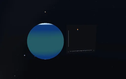
Ice and albedo feedback — Actual application image
Actual application image

What happens

Sixty latitude bands in x = sin(latitude) over one hemisphere. Each absorbs Q s(x)(1 − alpha(T)) with Q = 340 W/m² times the sunshine factor and North’s s = 1 − 0.482 P2(x), radiates A + B T with A = 203.3 W/m² and B = 2.09 W/m²·K, and exchanges heat by diffusion d/dx (D (1 − x²) dT/dx) with D = 0.40. The albedo turns from 0.30 for water to 0.62 for ice over a tanh range around −10 °C. Implicit steps of 0.05 year in diffusion and radiation, explicit in the albedo, a heat capacity of a 100 m mixed layer. With a constant albedo the equilibrium is the P2 solution; with the feedback the ice line jumps and the climate has two branches.

Try this

Read today’s ice edge; dim the sun or press the sweep and watch the snowball come; brighten it again and see how far the frozen branch holds; make the albedos equal and compare with the P2 solution.

The model and its limits

A zonally averaged, diffusive energy balance with a fixed outgoing law, no seasons, ocean dynamics or clouds; the thresholds belong to this idealized planet, not to the Earth’s history.

Equations used in the module
Equations
C·dT/dt = Q·s(x)·(1 − α(T)) − (A + B·T) + d/dx(D·(1 − x²)·dT/dx)
s(x) = 1 − 0.482·P2(x),  α = α_i + (α_w − α_i)·(1 + tanh((T − T_f)/ΔT))/2
T(x) = (Q·(1 − α) − A)/B − 0.482·Q·(1 − α)·P2(x)/(B + 6D)
x_s = sin φ_ice:  two stable branches, a snowball below Q_c
Related experiments

Back to catalogue
Carbon through Earth systems — Actual application image

Earth

Carbon through Earth systems

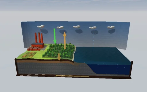
Follow every petagram of carbon through a museum relief of the Earth: chimneys burn fossil carbon into the air, the forest draws it down and drops it into the soil, the soil breathes it back faster as the world warms, and the ocean dissolves it - first the thin surface layer, whose buffer chemistry takes only a tenth of what its size suggests (the Revelle factor), then over centuries the deep ocean. Replay the industrial era: 667 PgC by 2025 bring CO2 to 426 ppm with 47 % still airborne; hold the emissions and CO2 passes 580 ppm by 2100, reach net zero in 2050 and it falls back towards 329 ppm. Release the same carbon at once or over two centuries, clear the forest, and watch the cycle share it out again: the multi-exponential response of the linearised cycle, its equilibrium partition and an exact carbon ledger are shown beside it.

Ocean carbonate chemistry — Actual application image

Earth

Ocean carbonate chemistry

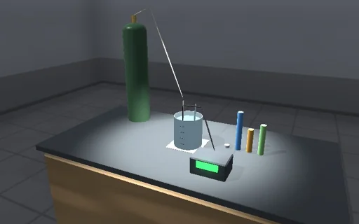
Bubble air of a chosen CO2 through a beaker of seawater on a laboratory bench and watch the indicator change colour. The water’s dissolved carbon and alkalinity fix its pH and the shares of dissolved CO2, bicarbonate and carbonate ion, with the published constants of Lueker, Dickson, Millero, Weiss and Mucci; the Revelle factor says why the water’s CO2 pressure rises ten times faster than its carbon. Raise the air’s CO2 and the carbonate ion falls until, near four thousand micro-atmospheres, the water can no longer keep aragonite: the shell on the bottom begins to dissolve, and its two units of alkalinity for every carbon buffer the water back to just under saturation. Cold water of the same chemistry holds less carbonate. Carbon in water, shell and air is conserved to rounding.