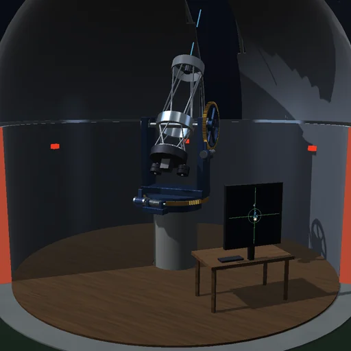
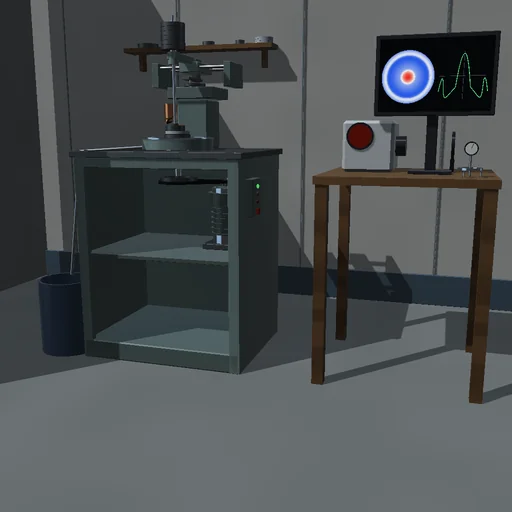
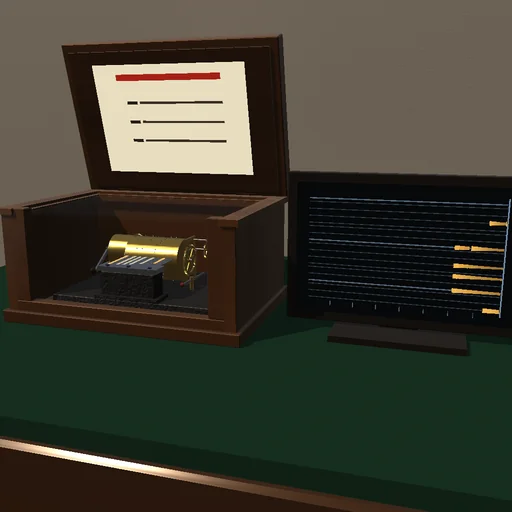
Engineering
Precision wafer stage
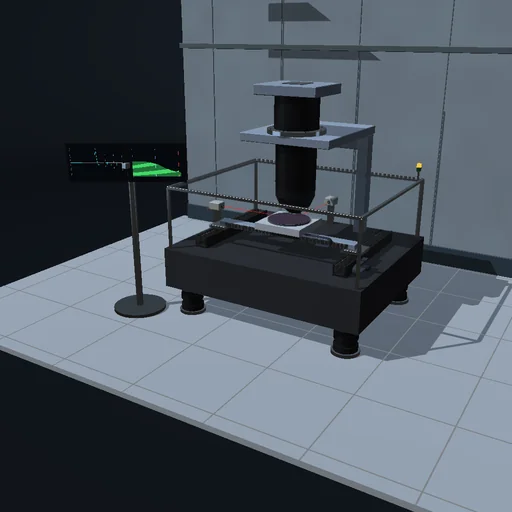
Step a 300 mm wafer under the lens field by field and watch the nanometre error settle on the console before each exposure. Compare the trapezoid with the S-curve, switch off the feedforward, soften the flexure until the loop rings and lower the bandwidth, load a heavier table and tune the controller to it, and shake the floor.
What happens
The wafer stage of a lithography stepper carries a 300 mm wafer under the projection lens and exposes it field by field: 83 fields of 26 × 33 mm in serpentine rows. Each axis of the H-drive is two masses: a carriage, 12 kg on X and 40 kg on Y with the beam, pushed by a linear motor of at most 1000 N (2400 N on Y), and the 8 kg wafer table on a flexure that resonates at 1027 Hz (the soft flexure at 398 Hz). An interferometer reads the table in counts of 1 nm. A digital PID at 10 kHz with a low-pass, its gains set by the bandwidth and by the mass it is tuned for, adds a feedforward of mass times the profile's acceleration. The profiles reach 0.5 m/s and 25 m/s², as a trapezoid or as an S-curve limited to 2500 m/s³; a field is exposed for 20 ms once both errors have stayed within ±10 nm for 1 ms.
The S-curve step lasts 82 ms; its error peaks at 112 nm and settles 10.0 ms after the profile: a cycle of 112.9 ms, 31887 fields an hour, the wafer in 9.47 s. The trapezoid moves 10 ms faster, but its steps of force ring the flexure for 30 ms. Without the feedforward the table lags 154 µm and the integral's tail takes 94.8 ms to settle. The soft flexure is unstable at the default 100 Hz: its mode grows into the force limit, and after 200 ms the stage exposes a field smeared over 38 µm. At 60 Hz it settles in 23.3 ms, but its slow tail returns and the field lands 29 nm off; at 40 Hz it settles cleanly in 42.5 ms. A 16 kg table on a controller tuned for 8 kg lags 64 µm and settles in 92.9 ms; tuned to it, in 10.7 ms. A floor vibration of 20 mm/s² moves the standing table 171 nm at 20 Hz, 62 nm at 100 Hz, 3.9 nm at 400 Hz. The reading differs from the true position by q/√12: 0.29 nm for a 1 nm count.
Model: rigid carriage and table joined by one flexure per axis; no yaw, tilt or coupling of the axes; a cable slab's spring and the air bearings' drag, both fed forward; the floor's vibration as an acceleration of the base along X. RK4 in sub-steps of 12.5 µs under the controller's zero-order hold; the controller keeps its own clock whatever the frame rate, and the sampled loop agrees with its exact discretization. The energy journal closes: motors and floor = kinetic energy, flexures, cable slabs, flexure damping and air-bearing drag. No motor ripple, thermal drift or wafer exchange; a model of the principle, not the nanometre claim of a real machine.
Try this
Watch the error settle on the console after each step, then switch to the trapezoid and see the ringing cost time. Switch off the feedforward, choose the soft flexure and lower the bandwidth until it holds, load a heavier table and tune the controller to it.
Equations used in the module
Equations
M₁·x₁″ = F − k·(x₁ − x₂) − c·(x₁′ − x₂′) − k_c·x₁ − b·x₁′ − M₁·a_f
M₂·x₂″ = k·(x₁ − x₂) + c·(x₁′ − x₂′) − M₂·a_f
F = LP²[K_p·e + K_i·Σe·T + K_d·Δe/T] + M_t·a_ref + b·v_ref + k_c·x_ref,  e = r − q·round(x₂/q)
K_p = M_t·ω_c²/3,  K_d = M_t·ω_c,  K_i = M_t·ω_c³/30;  f_r = √(k·(M₁ + M₂)/(M₁·M₂))/2π