Earth
Warm and cold fronts
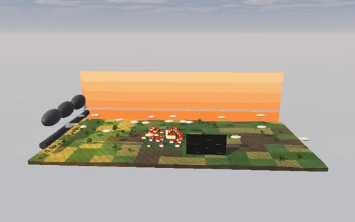
Watch a cold front pass over a small town on a hazy summer afternoon. Cold air, seven degrees colder and two kilometres deep, is released from the west and runs under the warm air as a density current: its nose moves at Benjamin’s Fr·√(g’h) on top of the steering wind, with the depth behind it and the speed both as Rottman and Simpson’s closed form says, and Ritter’s fan behind. The warm boundary layer is lifted over the cold air; above its condensation level it makes a dark shelf cloud with a roll cloud along the nose and a rain curtain behind. The town’s weather mast and meteogram record the temperature drop, the pressure jump ρg’h, the gust and the veering wind. Switch to Margules’ geostrophic fronts, tilted at f·Δv·T/(gΔT): a cold front carried by the wind, or a warm front with rain ahead and falling pressure. Without a density contrast nothing moves at all.
What happens
A vertical section across the front, uniform along it, x to the east. Cold air at T_w − 7 K under warm air at 26 °C is a reduced-gravity shallow-water layer, g’ = gΔT/T_w = 0.230 m/s², in 319 Lagrangian columns of fixed volume (250 m near the lock, wider back to a wall 300 km behind); the column pressures g’h²/2, an eddy viscosity of 2000 m²/s and a quadratic viscosity push the nodes in 2 s symplectic steps, Coriolis at 48° N acts on the along-front wind’s departure from the warm air’s, and every node keeps its absolute momentum v + f(x − u_b t). A 2 km reservoir released at x = 0 runs east under a 6 km deep warm layer with the nose at u_b + Fr(h/H)√(g’h), Benjamin’s Fr = √((2 − a)(1 − a)/(1 + a)); Rottman and Simpson: u + 2c = 2c0 with u = Fr c gives h_f = 781 m and U = 16.07 m/s, so with the 5 m/s steering wind the front reaches the town 36 km away in 28.5 min, and Ritter’s fan h = (2c0 − ξ)²/(9g’) lies behind. Margules’ fronts are wedges at tan α = fΔvT/(gΔT) = 5.7 m/km for a shear of 12 m/s, in exact discrete geostrophic balance and carried by the steering wind. The warm boundary layer, 1000 m deep at 65 % humidity, condenses above its LCL of 894 m (bisection along the dry adiabat with Magnus; closed form 889 m, Espy 885 m) at ρ·Γq per metre of lift and of saturated depth, Γq = 2.17 g/kg/km of the moist adiabat; 81 gauges take the condensation of the warm air passing over them and let it fall out over 15 min. The station records temperature, the hydrostatic pressure jump ρ_c g’h, wind and rain each minute.
Try this
Watch the front reach the town and the meteogram step: cold, pressure up by ρ_c g’h_f, a gust and a veer; compare the nose speed and the head with the closed form; switch off rotation and the agreement becomes exact; raise the humidity or the boundary layer for a darker shelf cloud and more rain; switch to Margules’ cold front for a veer from south to north-west, or to the warm front for rain ahead of it and falling pressure; take the rotation away from a Margules front and watch it slump; set the contrast low and it barely moves.
The model and its limits
Hydrostatic two-fluid layer under deep, passive warm air: no head billows, no mixing across the interface and no return flow; the finite depth of the warm air enters only through Benjamin’s front condition. The warm air is lifted exactly as far as the cold air beneath it is deep and condenses on a linearised moist adiabat; there is no convection, so the rain is that of layer lifting only, smaller than a real squall line’s, and it falls where it forms after a delay, without drift. The Margules wedges stop at the cold depth against a wall moving with the steering wind, far out of view; their surface tip node carries the mean of the two winds. Time steps are first order: the energy budget closes to about 10^-4 of the initial energy, volumes and absolute momentum to round-off. The town, trees, mast and board are not to scale.
Equations used in the module
Equations
∂h/∂t + ∂(h·u)/∂x = 0,  Du/Dt − f·(v − v_w) = −g’·∂h/∂x,  Dv/Dt = −f·(u − u_b),  g’ = g·ΔT/T_w
Nose: u_N = u_b + Fr·√(g’·h),  Fr = √((2 − a)(1 − a)/(1 + a)), a = h/H;  u + 2c = 2c0 ⇒ c_f = 2c0/(2 + Fr), h = (2c0 − x/t)²/(9g’) in Ritter’s fan
Margules: tan α = f·Δv·T/(g·ΔT);  Δp = ρ_c·g’·h
z_LCL = (T − T_d)/(g/c_p − g·R_v·T_d²/(L·R_d·T)),  C(Δz) = ρ·Γq·∫₀^D [max(0, z₀ + Δz − z_LCL) − max(0, z₀ − z_LCL)] dz₀